Bayesian edge selection or Bayesian estimation for a Markov random field model for binary and/or ordinal variables.

The function bgm explores the joint pseudoposterior distribution of parameters and possibly edge indicators for a Markov Random Field model for mixed binary and ordinal variables.

Usage

bgm(
  x,
  variable_type = "ordinal",
  reference_category,
  iter = 10000,
  burnin = 500,
  interaction_scale = 2.5,
  threshold_alpha = 0.5,
  threshold_beta = 0.5,
  edge_selection = TRUE,
  edge_prior = c("Bernoulli", "Beta-Bernoulli", "Stochastic-Block"),
  inclusion_probability = 0.5,
  beta_bernoulli_alpha = 1,
  beta_bernoulli_beta = 1,
  dirichlet_alpha = 1,
  na.action = c("listwise", "impute"),
  save = FALSE,
  display_progress = TRUE
)

Arguments

x: A data frame or matrix with n rows and p columns containing binary and ordinal variables for n independent observations and p variables in the network. Regular binary and ordinal variables are recoded as non-negative integers (0, 1, ..., m) if not already done. Unobserved categories are collapsed into other categories after recoding (i.e., if category 1 is unobserved, the data are recoded from (0, 2) to (0, 1)). Blume-Capel ordinal variables are also coded as non-negative integers if not already done. However, since “distance” to the reference category plays an important role in this model, unobserved categories are not collapsed after recoding.
variable_type: What kind of variables are there in x? Can be a single character string specifying the variable type of all p variables at once or a vector of character strings of length p specifying the type for each variable in x separately. Currently, bgm supports “ordinal” and “blume-capel”. Binary variables are automatically treated as “ordinal’’. Defaults to variable_type = "ordinal".
reference_category: The reference category in the Blume-Capel model. Should be an integer within the range of integer scores observed for the “blume-capel” variable. Can be a single number specifying the reference category for all Blume-Capel variables at once, or a vector of length p where the i-th element contains the reference category for variable i if it is Blume-Capel, and bgm ignores its elements for other variable types. The value of the reference category is also recoded when bgm recodes the corresponding observations. Only required if there is at least one variable of type “blume-capel”.
iter: How many iterations should the Gibbs sampler run? The default of 1e4 is for illustrative purposes. For stable estimates, it is recommended to run the Gibbs sampler for at least 1e5 iterations.
burnin: The number of iterations of the Gibbs sampler before saving its output. Since it may take some time for the Gibbs sampler to converge to the posterior distribution, it is recommended not to set this number too low. When edge_selection = TRUE, the bgm function will perform 2 * burnin iterations, first burnin iterations without edge selection, then burnin iterations with edge selection. This helps ensure that the Markov chain used for estimation starts with good parameter values and that the adaptive MH proposals are properly calibrated.
interaction_scale: The scale of the Cauchy distribution that is used as a prior for the pairwise interaction parameters. Defaults to 2.5.
threshold_alpha, threshold_beta: The shape parameters of the beta-prime prior density for the threshold parameters. Must be positive values. If the two values are equal, the prior density is symmetric about zero. If threshold_beta is greater than threshold_alpha, the distribution is skewed to the left, and if threshold_beta is less than threshold_alpha, it is skewed to the right. Smaller values tend to lead to more diffuse prior distributions.
edge_selection: Should the function perform Bayesian edge selection on the edges of the MRF in addition to estimating its parameters (edge_selection = TRUE), or should it just estimate the parameters (edge_selection = FALSE)? The default is edge_selection = TRUE.
edge_prior: The inclusion or exclusion of individual edges in the network is modeled with binary indicator variables that capture the structure of the network. The argument edge_prior is used to set a prior distribution for the edge indicator variables, i.e., the structure of the network. Currently, three options are implemented: The Bernoulli model edge_prior = "Bernoulli" assumes that the probability that an edge between two variables is included is equal to inclusion_probability and independent of other edges or variables. When inclusion_probability = 0.5, this means that each possible network structure is given the same prior weight. The Beta-Bernoulli model edge_prior = "Beta-Bernoulli" assumes a beta prior for the unknown inclusion probability with shape parameters beta_bernoulli_alpha and beta_bernoulli_beta. If beta_bernoulli_alpha = 1 and beta_bernoulli_beta = 1, this means that networks with the same complexity (number of edges) get the same prior weight. The Stochastic Block model edge_prior = "Stochastic-Block" assumes that nodes can be organized into blocks or clusters. In principle, the assignment of nodes to such clusters is unknown, and the model as implemented here considers all possible options @i.e., specifies a Dirichlet prior on the probability of allocations as described by @GengEtAl_2019bgms. This model is advantageous when nodes are expected to fall into distinct clusters. The inclusion probabilities for the edges are defined at the level of the clusters, with a beta prior for the unknown inclusion probability with shape parameters beta_bernoulli_alpha and beta_bernoulli_beta, and a Dirichlet prior on the cluster assignment probabilities with a common concentration parameter dirichlet_alpha. The default is edge_prior = "Bernoulli".
inclusion_probability: The prior edge inclusion probability for the Bernoulli model. Can be a single probability, or a matrix of p rows and p columns specifying an inclusion probability for each edge pair. The default is inclusion_probability = 0.5.
beta_bernoulli_alpha, beta_bernoulli_beta: The two shape parameters of the Beta prior density for the Bernoulli inclusion probability. Must be positive numbers. Defaults to beta_bernoulli_alpha = 1 and beta_bernoulli_beta = 1.
dirichlet_alpha: The shape of the Dirichlet prior on the node-to-block allocation probabilities for the Stochastic Block model.
na.action: How do you want the function to handle missing data? If na.action = "listwise", listwise deletion is used. If na.action = "impute", missing data are imputed iteratively during the MCMC procedure. Since imputation of missing data can have a negative impact on the convergence speed of the MCMC procedure, it is recommended to run the MCMC for more iterations. Also, since the numerical routines that search for the mode of the posterior do not have an imputation option, the bgm function will automatically switch to interaction_prior = "Cauchy" and adaptive = TRUE.
save: Should the function collect and return all samples from the Gibbs sampler (save = TRUE)? Or should it only return the (model-averaged) posterior means (save = FALSE)? Defaults to FALSE.
display_progress: Should the function show a progress bar (display_progress = TRUE)? Or not (display_progress = FALSE)? The default is TRUE.

Value

If save = FALSE (the default), the result is a list of class “bgms” containing the following matrices with model-averaged quantities:

indicator: A matrix with p rows and p columns, containing the posterior inclusion probabilities of individual edges.
interactions: A matrix with p rows and p columns, containing model-averaged posterior means of the pairwise associations.
thresholds: A matrix with p rows and max(m) columns, containing model-averaged category thresholds. In the case of “blume-capel” variables, the first entry is the parameter for the linear effect and the second entry is the parameter for the quadratic effect, which models the offset to the reference category.
In the case of edge_prior = "Stochastic-Block" two additional elements are returned: a vector allocations with the estimated cluster assignments of the nodes and an table clusters with the estimated posterior probability of the number of clusters in the network. The vector of node allocations is calculated using a method proposed by Dahl2009bgms and also used by GengEtAl_2019bgms.

If save = TRUE, the result is a list of class “bgms” containing:

indicator: A matrix with iter rows and p * (p - 1) / 2 columns, containing the edge inclusion indicators from every iteration of the Gibbs sampler.
interactions: A matrix with iter rows and p * (p - 1) / 2 columns, containing parameter states from every iteration of the Gibbs sampler for the pairwise associations.
thresholds: A matrix with iter rows and sum(m) columns, containing parameter states from every iteration of the Gibbs sampler for the category thresholds.
In the case of edge_prior = "Stochastic-Block" a matrix allocations with the cluster assignments of the nodes from each iteration is returned. This matrix can be used to calculate the posterior probability of the number of clusters by utilizing the summary_SBM(bgm_output[["allocations"]]) function.

Column averages of these matrices provide the model-averaged posterior means. Except for the allocations matrix, for which the summary_SBM needs to be utilized.

In addition to the analysis results, the bgm output lists some of the arguments of its call. This is useful for post-processing the results.

Details

Currently, bgm supports two types of ordinal variables. The regular, default, ordinal variable type has no restrictions on its distribution. Every response category except the first receives its own threshold parameter. The Blume-Capel ordinal variable assumes that there is a specific reference category, such as the “neutral” in a Likert scale, and responses are scored in terms of their distance to this reference category. Specifically, the Blume-Capel model specifies the following quadratic model for the threshold parameters: $$\mu_{\text{c}} = \alpha \times \text{c} + \beta \times (\text{c} - \text{r})^2,$$ where $\mu_{\text{c}}$ is the threshold for category c. The parameter $\alpha$ models a linear trend across categories, such that $\alpha > 0$ leads to an increasing number of observations in higher response categories and $\alpha <0$ leads to a decreasing number of observations in higher response categories. The parameter $\beta$ models the response style in terms of an offset with respect to the reference category $r$; if $\beta<0$ there is a preference to respond in the reference category (i.e., the model introduces a penalty for responding in a category further away from the reference_category category r), while if $\beta > 0$ there is preference to score in the extreme categories further away from the reference_category category.

The Bayesian estimation procedure (edge_selection = FALSE) simply estimates the threshold and pairwise interaction parameters of the ordinal MRF, while the Bayesian edge selection procedure (edge_selection = TRUE) also models the probability that individual edges should be included or excluded from the model. Bayesian edge selection imposes a discrete spike and slab prior distribution on the pairwise interactions. By formulating it as a mixture of mutually singular distributions, the function can use a combination of Metropolis-Hastings and Gibbs sampling to create a Markov chain that has the joint posterior distribution as an invariant. The current option for the slab distribution is a Cauchy with an optional scaling parameter. The slab distribution is also used as the prior for the interaction parameters for Bayesian estimation. A beta-prime distribution is used for the exponent of the category parameters. For Bayesian edge selection, two prior distributions are implemented for the edge inclusion variables (i.e., the prior probability that an edge is included); the Bernoulli prior and the Beta-Bernoulli prior.

References

Examples

# \donttest{
 #Store user par() settings
 op <- par(no.readonly = TRUE)

 ##Analyse the Wenchuan dataset

 # Here, we use 1e4 iterations, for an actual analysis please use at least
 # 1e5 iterations.
 fit = bgm(x = Wenchuan)
#> Warning: There were 18 rows with missing observations in the input matrix x.
#> Since na.action = listwise these rows were excluded from the analysis.


 #------------------------------------------------------------------------------|
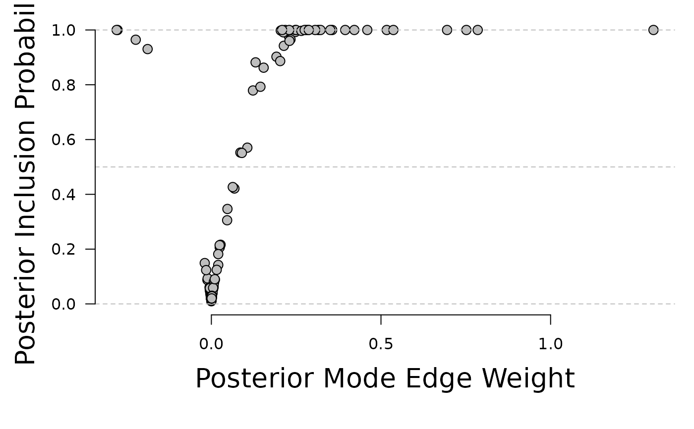
 # INCLUSION - EDGE WEIGHT PLOT
 #------------------------------------------------------------------------------|

 par(mar = c(6, 5, 1, 1))
 plot(x = fit$interactions[lower.tri(fit$interactions)],
      y = fit$indicator[lower.tri(fit$indicator)], ylim = c(0, 1),
      xlab = "", ylab = "", axes = FALSE, pch = 21, bg = "gray", cex = 1.3)
 abline(h = 0, lty = 2, col = "gray")
 abline(h = 1, lty = 2, col = "gray")
 abline(h = .5, lty = 2, col = "gray")
 mtext("Posterior Mode Edge Weight", side = 1, line = 3, cex = 1.7)
 mtext("Posterior Inclusion Probability", side = 2, line = 3, cex = 1.7)
 axis(1)
 axis(2, las = 1)



 #------------------------------------------------------------------------------|
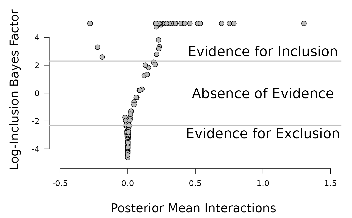
 # EVIDENCE - EDGE WEIGHT PLOT
 #------------------------------------------------------------------------------|

 #For the default choice of the structure prior, the prior odds equal one:
 prior.odds = 1
 posterior.inclusion = fit$indicator[lower.tri(fit$indicator)]
 posterior.odds = posterior.inclusion / (1 - posterior.inclusion)
 log.bayesfactor = log(posterior.odds / prior.odds)
 log.bayesfactor[log.bayesfactor > 5] = 5

 par(mar = c(5, 5, 1, 1) + 0.1)
 plot(fit$interactions[lower.tri(fit$interactions)], log.bayesfactor, pch = 21, bg = "#bfbfbf",
      cex = 1.3, axes = FALSE, xlab = "", ylab = "", ylim = c(-5, 5.5),
      xlim = c(-0.5, 1.5))
 axis(1)
 axis(2, las = 1)
 abline(h = log(1/10), lwd = 2, col = "#bfbfbf")
 abline(h = log(10), lwd = 2, col = "#bfbfbf")

 text(x = 1, y = log(1 / 10), labels = "Evidence for Exclusion", pos = 1,
      cex = 1.7)
 text(x = 1, y = log(10), labels = "Evidence for Inclusion", pos = 3, cex = 1.7)
 text(x = 1, y = 0, labels = "Absence of Evidence", cex = 1.7)
 mtext("Log-Inclusion Bayes Factor", side = 2, line = 3, cex = 1.5, las = 0)
 mtext("Posterior Mean Interactions ", side = 1, line = 3.7, cex = 1.5, las = 0)



 #------------------------------------------------------------------------------|
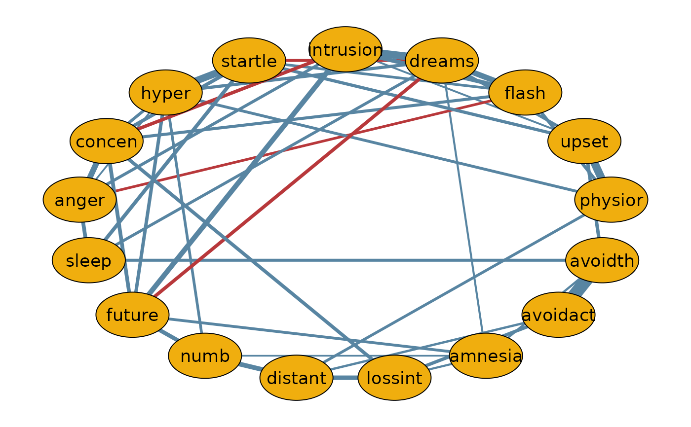
 # THE MEDIAN PROBABILITY NETWORK
 #------------------------------------------------------------------------------|

 tmp = fit$interactions[lower.tri(fit$interactions)]
 tmp[posterior.inclusion < 0.5] = 0

 median.prob.model = matrix(0, nrow = ncol(Wenchuan), ncol = ncol(Wenchuan))
 median.prob.model[lower.tri(median.prob.model)] = tmp
 median.prob.model = median.prob.model + t(median.prob.model)

 rownames(median.prob.model) = colnames(Wenchuan)
 colnames(median.prob.model) = colnames(Wenchuan)

 library(qgraph)
 qgraph(median.prob.model,
        theme = "TeamFortress",
        maximum = .5,
        fade = FALSE,
        color = c("#f0ae0e"), vsize = 10, repulsion = .9,
        label.cex = 1.1, label.scale = "FALSE",
        labels = colnames(Wenchuan))


 #Restore user par() settings
 par(op)
# }

References

Geng J, Bhattacharya A, Pati D (2019). “Probabilistic community detection with unknown number of communities.” Journal of the American Statistical Association, 114, 893–905. doi:10.1080/01621459.2018.1458618 .